How to Perform Feature Selection in Machine Learning

In this guide, you will learn multiple feature selection techniques with easy-to-follow Python examples.

Welcome to this fun and hands-on journey into the world of Feature Selection in Machine Learning (ML).

But first, what is feature selection?

Feature Selection

Feature selection is the process of selecting the most relevant features (columns) in your dataset to build a machine learning model.

Why?

Because sometimes, less is more — fewer features can also mean:

1. Faster computation.

2. Simpler models that are easier to interpret.

3. Better performance by removing noise.

4. Reduces complexity / risk of overfitting.

5. Reduces training time.

Techniques We’ll Cover:

1. Variance Thresholding — Eliminating features with low variance.

2. Correlation-based Selection — Dropping features that are highly correlated.

3. Recursive Feature Elimination (RFE) — Iteratively removing features to find the best subset.

4. Feature Importance — Leveraging random forest for ranking important features.

   
   

But before we implement these techniques, lets load the dataset.

Dataset: The Titanic Dataset

We’ll use the Titanic dataset because who doesn’t love a good historical tragedy mixed with machine learning? Also, almost all of us would be aware of this dataset, thanks to the movie!

# load the requires libraries
import seaborn as sns
import pandas as pd
from sklearn.model_selection import train_test_split

# Load Titanic dataset
data = sns.load_dataset('titanic')
data.head()

Output:

The next step is to perform data cleaning.

The steps we’ll do here are:

• Remove irrelevant and duplicate variables

• Drop missing values (other techniques are available but that’s not the main scope here)

• Encoding categorical variables

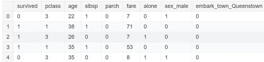
The following lines of code will perform the above steps and display the first five rows of the dataset.

# Drop irrelevant columns
data = data.drop(['deck', 'embarked', 'alive', 'who', 'adult_male', 'class'], axis=1)

# Handle missing values
data = data.dropna()

# Separate numerical and categorical columns

numerical_cols = data.select_dtypes(include=['int64', 'float64']).columns

categorical_cols = data.select_dtypes(include=['object']).columns # Encode categorical variables

# Encode categorical variables with dummy encoding (1 and 0)
data = pd.get_dummies(data, columns=categorical_cols, drop_first=True).astype(int)

data.head()

Output:

Okay, so we have got a lot of data cleaning and preprocessing done.

Let’s create the X and y arrays that indicates the independent and target variable, respectively.

Also, we’ll create the train and test set as well. This is done in the code below.

# Split features and target

X = data.drop('survived', axis=1)y = data['survived']

# Train-Test Split
X_train, X_test, y_train, y_test = train_test_split(X, y, test_size=0.3, random_state=10)

With this task done and dusted, we are now ready to explore the various feature selection techniques.

1. Variance Thresholding

Let’s start by removing features with low variance. Low variance means the feature doesn’t change much across observations, so it’s probably not very useful.

from sklearn.feature_selection import VarianceThreshold
selector = VarianceThreshold(threshold=0.1)
X_train_var = selector.fit_transform(X_train)

print("Original Features:", X_train.shape[1])
print("Features Remaining:", X_train_var.shape[1])

Output:

The number of features before and after applying variance thresholding value of 0.1.

So we can see that one feature has been eliminated at threshold of 0.1.

Let’s now keep the threshold at 0.3.

from sklearn.feature_selection import VarianceThreshold
selector = VarianceThreshold(threshold=0.3)

X_train_var2 = selector.fit_transform(X_train)

print("Original Features:", X_train.shape[1])
print("Features Remaining:", X_train_var2.shape[1])

Output:

This time, we have 5 features remaining. So the threshold value plays an important role in feature selection.

2. Correlation-based Selection

Highly correlated features can be redundant. Let’s drop one feature from each highly correlated pair.

The code below computes and displays the corrleation matrix of the numerical features.

import numpy as np

# Select numerical columns only for correlation analysis
numerical_cols_train = X_train.select_dtypes(include=['int64', 'float64']).columns

correlation_matrix = X_train[numerical_cols_train].corr().abs()

correlation_matrix

Output:

The alone variable has correlation above 0.6 with both sibsp and parch variables. Lets keep the value of 0.6 as the correlation threshold.

This is not a hard and fast rule, and you can keep a higher or lower threshold depending on your use case.

upper = correlation_matrix.where(np.triu(np.ones(correlation_matrix.shape), k=1).astype(bool))

# Drop features with correlation > 0.6
to_drop = [column for column in upper.columns if any(upper[column] > 0.6)]

X_train_corr = X_train.drop(columns=to_drop)

print("Dropped Columns:", to_drop)
print("Remaining Features:", X_train_corr.shape[1])

Output:

Names of columns dropped due to high correlation and the number of remaining features.

3. Recursive Feature Elimination (RFE)

RFE is like a game of musical chairs — features are removed iteratively until only the best remain.

The code below uses the RandomForestClassifier model to select and print the top 5 features.

from sklearn.feature_selection import RFE

from sklearn.ensemble import RandomForestClassifier

model = RandomForestClassifier()

rfe = RFE(model, n_features_to_select=5)

X_train_rfe = rfe.fit_transform(X_train, y_train)

print("Selected Features:", X_train.columns[rfe.support_].tolist())

Output:

The code above will generate the list of the top 5 features selected by RFE.

4. Feature Importance using Random Forest

Random Forest is also used in ranking features based on importance. Let’s use the code below to identify key features.

model = RandomForestClassifier()

model.fit(X_train, y_train)

importances = model.feature_importances_

feature_importances = pd.DataFrame({'Feature': X_train.columns, 'Importance': importances})

feature_importances = feature_importances.sort_values(by='Importance', ascending=False)

print(feature_importances)

Output:

A sorted table showing each feature’s importance score.

So the variables age , sex_male and fare are the 3 most important features. This is consistent with the above result.

To conclude:

Congratulations! You’ve just learned four powerful techniques to declutter your dataset and make your ML models more efficient.

But Remember:

• Not all features deserve a spot in your final model — keep only the most important ones that add predictive power to your model.

• Feature selection is part art, part science — so experiment and iterate.

Got questions? Comments? Or just want to share your Titanic survival predictions? Drop them below!

Happy Learning!